# How to Diagnose Overfitting and Underfitting Here are some notes on analyzing overfitting and underfitting. ## Solutions to Overfitting Here are some common solutions to reduce generalization error: - Collect more training data Collecting more training data is often not applicable. - Simplify the model We can choose a simpler model with fewer parameters - Regularization Regularization helps a model to choose between two models with the same accuracy. If you obtain the same accuracy with a complex model as with a simple model, you should choose the simpler model. This principle is often referred to as Occam’s razor, the KISS principle, and more. The goal of regularization is to change the cost function in order to make model complexity an additional cost. In short, we introduce a penalty for complexity via regularization. - Data augmentation Data augmentation is a task that is very often used in ML for image treatment. It is easy to augment image data by adding slightly transformed images to your train data set. Examples are: Many functions exist for data augmentation on images such as the Tensorflow data augmentation layers. For tabular data, data augmentation includes oversampling and undersampling techniques such as SMOTE. - Reduce the dimensionality of the data In the next chapter, we will learn about a useful technique to check whether more training data is helpful. Here we look at some ways to reduce overfitting using regularization and dimensionality reduction via feature selection. Another useful approach to select relevant features from a dataset is to use a random forest which is an ensemble technique. - Hyperparameter tuning with cross-validation Hyperparameter tuning is the task of adjusting the model hyperparameters to improve model performance. The simplest approach is to use a grid search which involves testing out multiple combinations of hyperparameter values and evaluating their performance using cross-validation. This, we can find the hyperparameter combination that yields the best cross-validation score. - Ensemble models Random Forests claim not ro overfit but practice this is debatable. However, it is safe to say that ensemble can be a great help in avoiding overfitting. An ensemble model is the art of putting multiple weak learners together. The new prediction is the average prediction of all of those weak learners. We can create an ensemble by grouping multiple models into an ensemble wrapper: Voting Classifier: For multiple classification models the most often predicted class will be retained. Voting Regressor: Takes the average prediction of all individual models to make a prediction for a numerical target. Stacking Classifier: Build an additional classification model that uses the predictions of each individual model as an input and predicts the final target. Stacking Regressor: Build an additional regression model that uses the predictions of each individual model as an input for a final regression model that combines them into a final prediction. ## Principles of Overfitting and Underfitting ### Bias/Variance Trade-off _Underfitting_ is when your model is too simple for your data (high bias). _Overfitting_ is when your model is too complex for your data (high variance) but does not generalize well to new data. In the bias/variance trade-off, here are possible values: - low bias, low variance: a good result. - high bias, low variance (underfitting): the algorithm outputs similar predictions for similar data but predictions are wrong. - low bias, high variance (overfitting): the algorithm outputs very different predictions for similar data. - high bias, high variance: very bad algorithm (rare occurance). _Variance_ measures the consistency or variability of the model prediction for a particular sample instance if we were to retrain the model multiple times using different subsets of the training dataset. Thus, we say that the model is sensitive to the _randomness_ in the training data. _Bias_ measures how far off the predictions are from the correct values on average if we rebuild the model multiple times on different training datasets. Thus, bias is the measure of the _error_ that is not due to randomness. ### How to Detect Underfitting and Overfitting Underfitting means that your model makes accurate but incorrect predictions. In this case, train error is large and val/test error is large too. Overfitting means that your model makes not accurate predictions. In this case, train error is small and val/test error is large. When you find a good model, train error is small (but larger than in the case of overfitting) and val/test error is also small. NOTE: The train, validation, and test datasets should all have the same distribution. ### More Simple / Complex Model To complicate the model, you need to add more parameters called _degrees of freedom_ which means to try a more powerful model. If the algorithm is already quite complex (neural network or some ensemble model), you need to add more parameters to it such as increase the number of models in boosting. In the context of neural networks, this means adding more layers / more neurons in each layer / more connections between layers / more filters for CNN, and so on. To simplify the model, you need to reduce the number of parameters by changing the algorithm (such as random forest instead of deep neural network) or reduce the number of degrees of freedom. ### More Regularization / Less Regularization Regularization is an indirect and forced simplification of the model. The regularization term requires the model to keep parameters values as small as possible which requires the model to be as simple as possible. Complex models with strong regularization often perform better than simple models, so this is a very powerful tool. More regularization (simplifying the model) means increasing the impact of the regularization term which depends on the algorithm, so the regularization parameters are different. Thus, you should study the parameters of the algorithm and pay attention to whether they should be increased or decreased in a particular situation. There are a lot of such parameters — L1/L2 coefficients for linear regression, C and gamma for SVM, maximum tree depth for decision trees, and so on. In the context of neural networks, the main regularization methods are: - Early stopping - Dropout - L1 and L2 Regularization In the case when the model needs to be complicated, you should reduce the influence of regularization terms or use no regularization and see what happens. ### More Features / Fewer Features Adding new features also complicates the model. We can obtain new features for existing data is used infrequently, mainly due to the fact that it is very expensive and long but sometimes this can help. We can obtain artificial features from existing ones called _feature engineering_ which is often used for classical machine learning models. There are as many examples of such transformations but here are the main ones: - polynomial features — from x₁, x₂ to x₁, x₂, x₁x₂, x₁², x₂², ... (sklearn.preprocessing.PolynomialFeatures class) - log(x) for data with not-normal distribution - ln(|x| + 1) for data with heavy right tail - transformation of categorical features - other non-linear data transformation (from length and width to area (`length*width`) and so on. Linear models often work worse if some features are dependent — highly correlated. In this case, you need to use feature selection approaches to select only those features that carry the maximum amount of useful information. For neural networks, feature engineering and feature selection make almost no sense because the network finds dependencies in the data itself which is why deep neural networks can restore such complex dependencies. ### Why Getting More Data Sometimes Can’t Help One of the techniques to combat overfitting is to get more data. Surprisingly, this may not always help. Getting more data will not help in case of underfitting. Getting more data can help with overfitting (not underfitting) if the model is not too complex. Some tools such as data cleaning and cross-validation or hold-out validation are common practices in machine learning projects that can also be used to combat overfitting.  **Table:** Techniques to fight underfitting and overfitting (extended). ## Why is my validation loss lower than my training loss? In this tutorial, you will learn the three primary reasons your validation loss may be lower than your training loss when training your own custom deep neural networks. At the most basic level, a loss function quantifies how “good” or “bad” a given predictor is at classifying the input data points in a dataset. The smaller the loss, the better a job the classifier is at modeling the relationship between the input data and the output targets. However, there is a point where we can overfit our model — by modeling the training data too closely, our model loses the ability to generalize. Thus, we seek to: - Drive our loss down, improving our model accuracy. - Do so as fast as possible and with as little hyperparameter updates/experiments. - Avoid overfitting our network and modeling the training data too closely. It is a balancing act and our choice of loss function and model optimizer can dramatically impact the quality, accuracy, and generalizability of our final model. Typical loss functions (objective functions or scoring functions) include: - Binary cross-entropy - Categorical cross-entropy - Sparse categorical cross-entropy - Mean Squared Error (MSE) - Mean Absolute Error (MAE) - Standard Hinge - Squared Hinge For most tasks: - Loss measures the “goodness” of your model - The smaller the loss, the better - But careful not to overfit ### Reason 1: Regularization applied during training but not during validation/testing When training a deep neural network we often apply **regularization** to help our model: - Obtain higher validation/testing accuracy - To generalize better to the data outside the validation and testing sets Regularization methods often **sacrifice training accuracy to improve validation/testing accuracy** — in some cases this can lead to your validation loss being lower than your training loss. Also keep in mind that regularization methods such as dropout are not applied at validation/testing time. ### Reason 2: Training loss is measured during each epoch while validation loss is measured after each epoch The second reason you may see validation loss lower than training loss is due to how the loss value is measured and reported: - Training loss is measured _during_ each epoch - While validation loss is measured _after_ each epoch Your training loss is continually reported over the course of an entire epoch, but **validation metrics are computed over the validation set only once the current training epoch is completed**. Thus, on average the training losses are measured half an epoch earlier. ### Reason 3: The validation set may be easier than the training set (or there may be leaks) The third common reason is due to the data distribution itself. Consider how your validation set was acquired: - Can you guarantee that the validation set was sampled from the same distribution as the training set? - Are you certain that the validation examples are just as challenging as your training images? - Can you assure there was no _data leakage_ (training samples getting accidentally mixed in with validation/testing samples)? - Are you confident your code created the training, validation, and testing splits properly? Every deep learning practitioner has made the above mistakes at least once in their career. ## Diagnose Overfitting and Underfitting of LSTM Models It can be difficult to determine whether your Long Short-Term Memory model is performing well on your sequence prediction problem. You may be getting a good model skill score but it is important to know whether your model is a good fit for your data or if it is underfit or overfit and could do better with a different configuration. In this tutorial, you will discover how you can diagnose the fit of your LSTM model on your sequence prediction problem. After completing this tutorial, you will know: - How to gather and plot training history of LSTM models. - How to diagnose an underfit, good fit, and overfit model. - How to develop more robust diagnostics by averaging multiple model runs. ### Tutorial Overview This tutorial is divided into 6 parts: 1. Training History in Keras 2. Diagnostic Plots 3. Underfit Example 4. Good Fit Example 5. Overfit Example 6. Multiple Runs Example ### Training History in Keras You can learn a lot about the behavior of your model by reviewing its performance over time. LSTM models are trained by calling the `fit()` function which returns a variable called _history_ that contains a trace of the loss and any other metrics specified during the compilation of the model. Theae metric scores are recorded at the end of each epoch. ### Diagnostic Plots The training history of your LSTM models can be used to diagnose the behavior of your model. **Learning Curve:** Line plot of learning (y-axis) over experience (x-axis). During the training of a machine learning model, the current state of the model at each step of the training algorithm can be evaluated. It can be evaluated on the training dataset to give an idea of how well the model is learning. You can plot the performance of your model using the `matplotlib` library. - **Train Learning Curve:** Learning curve calculated from the training dataset that gives an idea of how well the model is learning. - **Validation Learning Curve:** Learning curve calculated from a hold-out validation dataset that gives an idea of how well the model is generalizing. It is common to create learning curves for multiple metrics such as in the case of classification predictive modeling problems, where the model may be optimized according to cross-entropy loss and model performance is evaluated using classification accuracy. In this case, two plots are created: one for the learning curves of each metric where each plot can show two learning curves (one for each of the train and validation datasets). - **Optimization Learning Curves:** Learning curves calculated on the metric by which the parameters of the model are being optimized such as loss. - **Performance Learning Curves:** Learning curves calculated on the metric by which the model will be evaluated and selected such as accuracy. 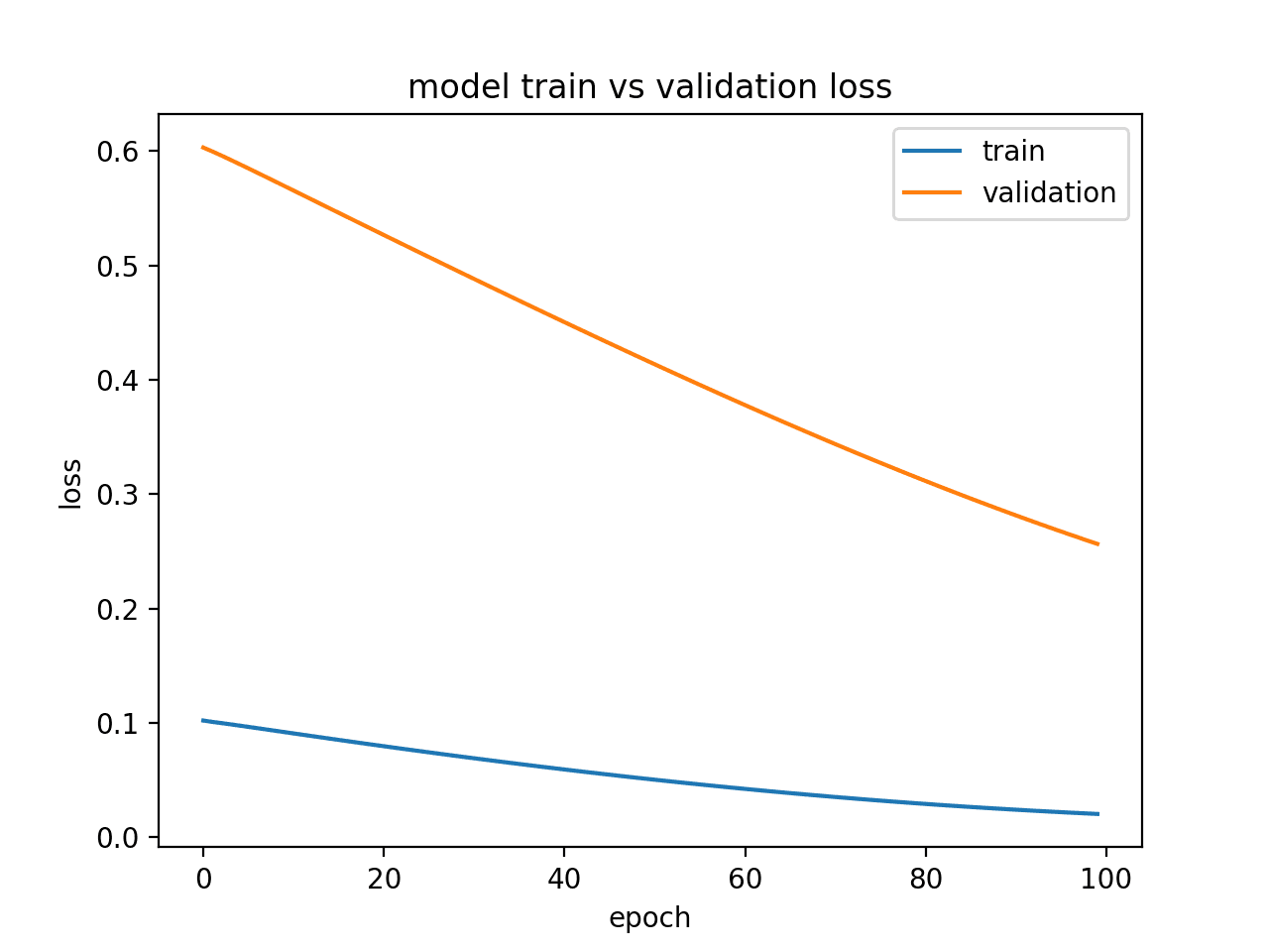### Underfit Example An underfit model is one that is demonstrated to perform well on the training dataset and poor on the test dataset. This can be diagnosed from a plot where the training loss is lower than the validation loss, and the validation loss has a trend that suggests further improvements are possible. 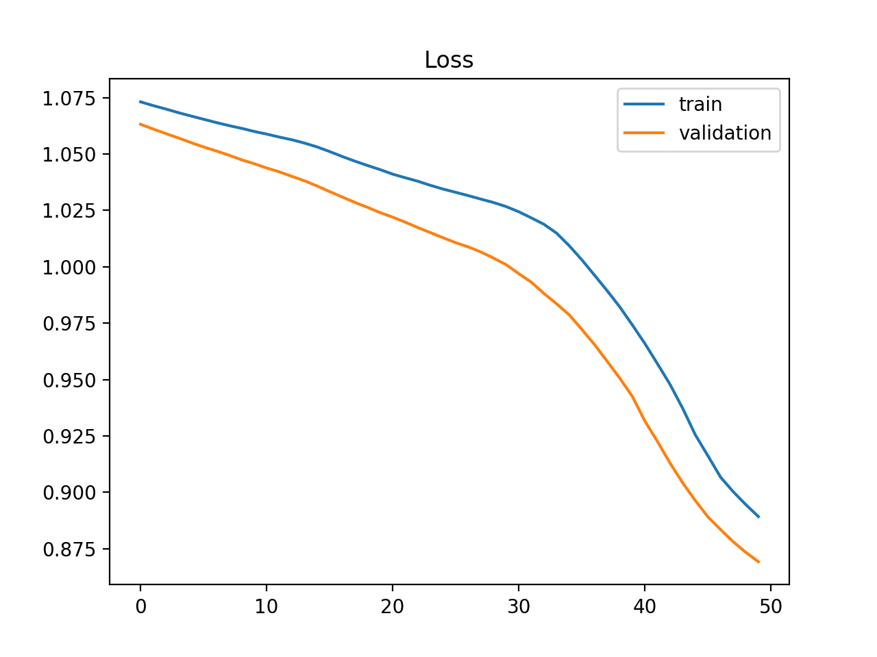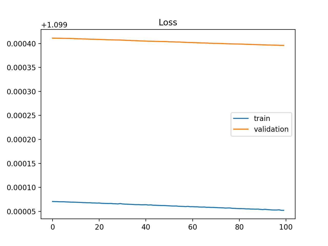#### Underfit Example 1  #### Underfit Example 2  #### Underfit Example 3  A plot of learning curves shows underfitting if: - The training loss remains flat regardless of training. - The training loss continues to decrease until the end of training. 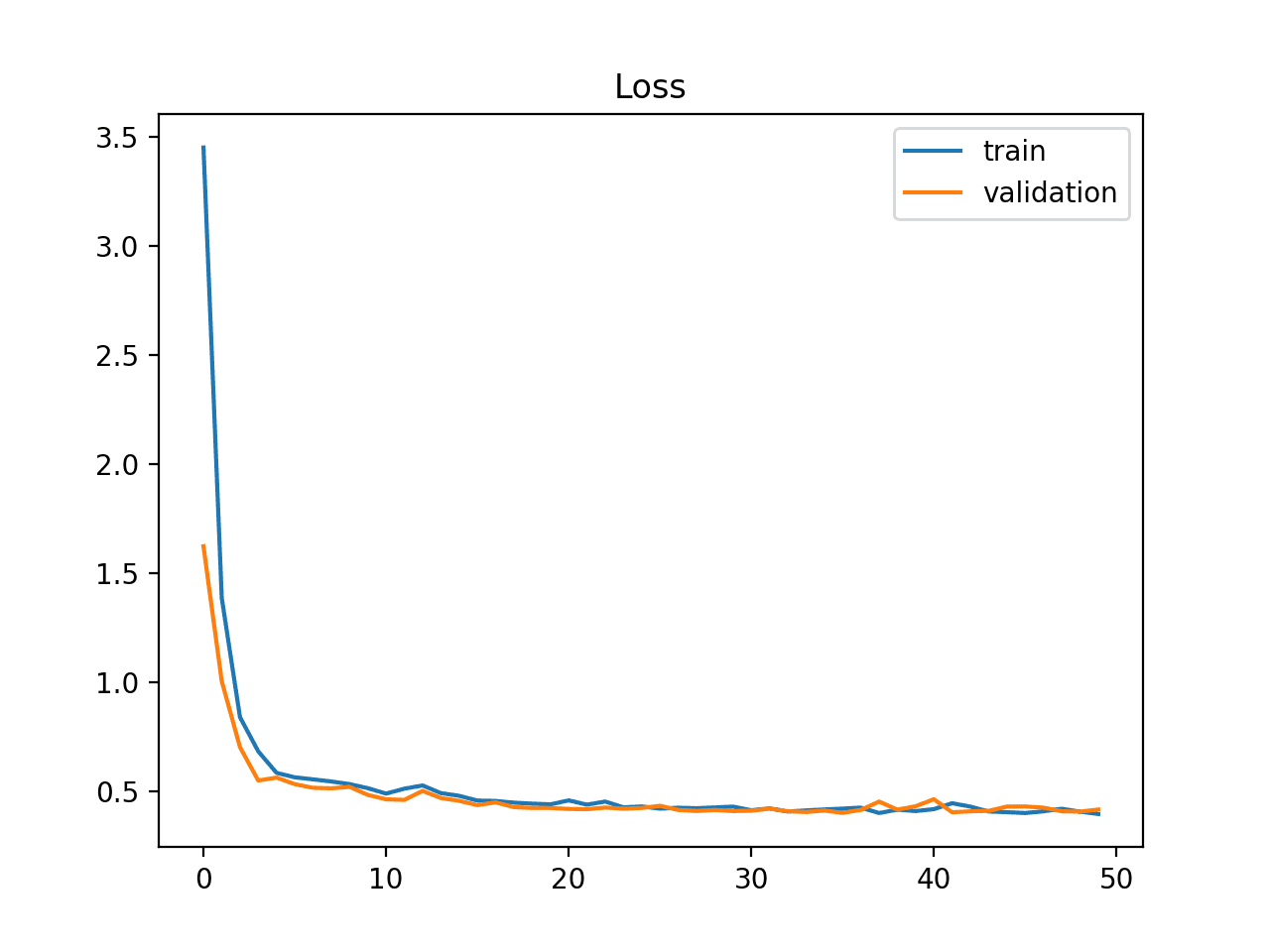### Good Fit Example A good fit is a case where the performance of the model is good on both the train and validation sets. This can be diagnosed from a plot where the train and validation loss decrease and stabilize around the same point. 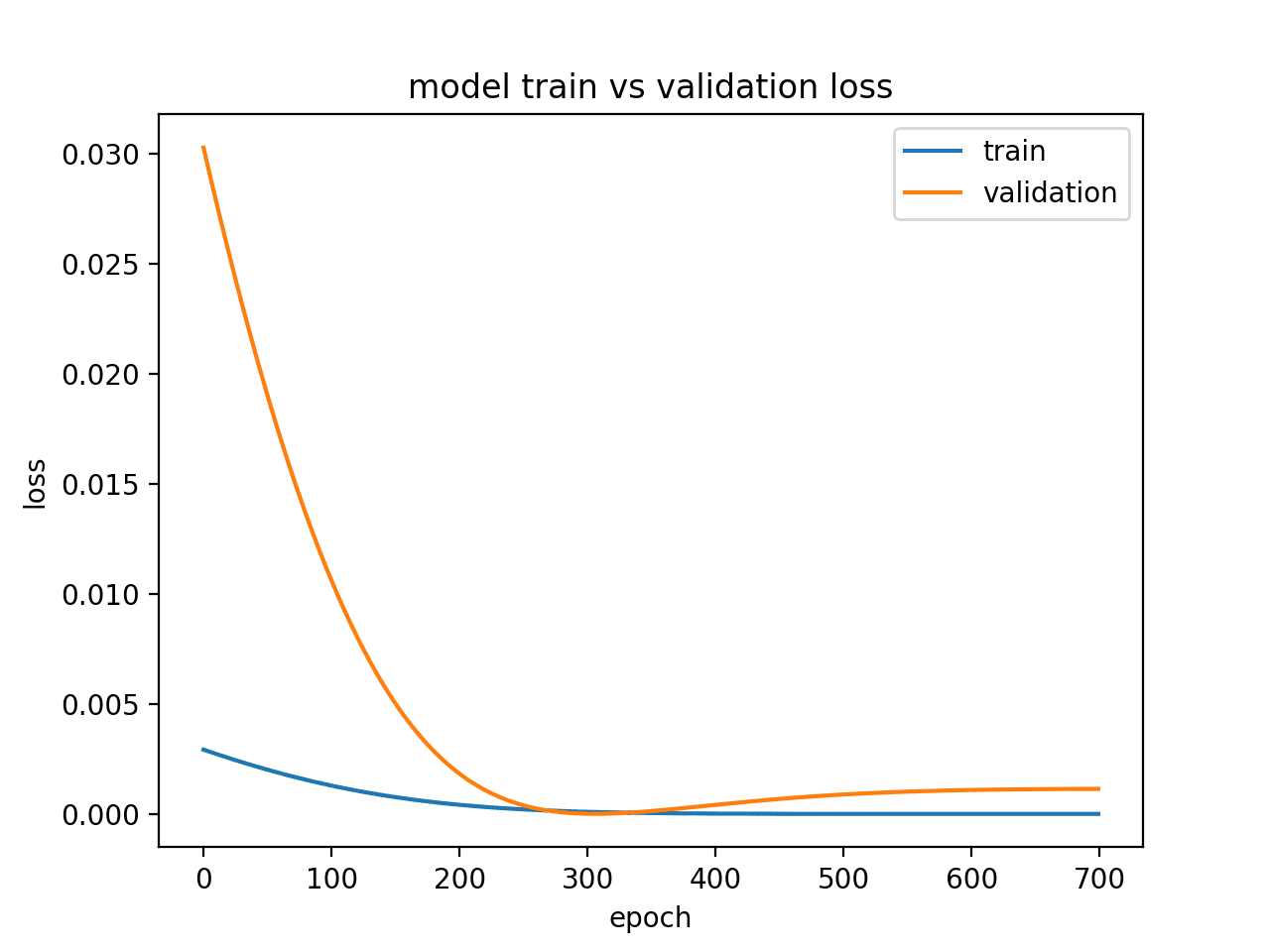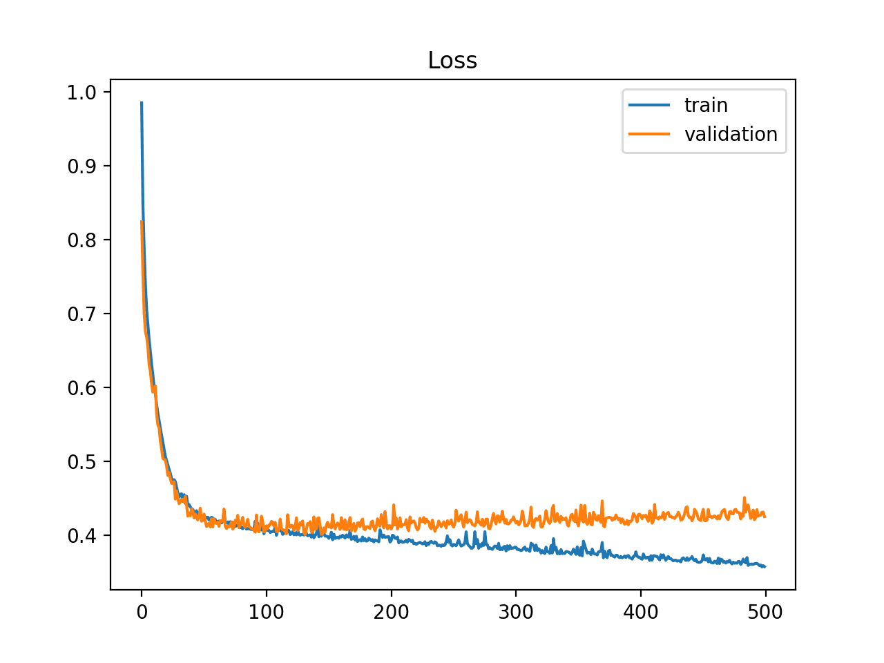#### Good Fit Example 1  #### Good Fit Example 2  ### Overfit Example An overfit model is one where performance on the train set is good and continues to improve whereas performance on the validation set improves to a point and then begins to degrade. This can be diagnosed from a plot where the train loss slopes down and the validation loss slopes down, hits an inflection point, and starts to slope up again. #### Underfit Example 1  #### Underfit Example 2  ### Multiple Runs Example LSTMs are stochastic which means that you will get a different diagnostic plot each run. It can be useful to repeat the diagnostic run multiple times (say 5, 10, or 30). The train and validation traces from each run can then be plotted to give a more robust idea of the behavior of the model over time. The example below runs the same experiment a number of times before plotting the trace of train and validation loss for each run. ## Diagnosing Unrepresentative Datasets Learning curves can also be used to diagnose properties of a dataset and whether it is relatively representative. An unrepresentative dataset means a dataset that may not capture the statistical characteristics relative to another dataset drawn from the same domain, such as between a train and a validation dataset. This can commonly occur if the number of samples in a dataset is too small, relative to another dataset. There are two common cases that could be observed; they are: - Training dataset is relatively unrepresentative. - Validation dataset is relatively unrepresentative. ### Unrepresentative Train Dataset An unrepresentative training dataset means that the training dataset does not provide sufficient information to learn the problem, relative to the validation dataset used to evaluate it. This may occur if the training dataset has too few examples as compared to the validation dataset. This situation can be identified by a learning curve for training loss that shows improvement and similarly a learning curve for validation loss that shows improvement, but a large gap remains between both curves.  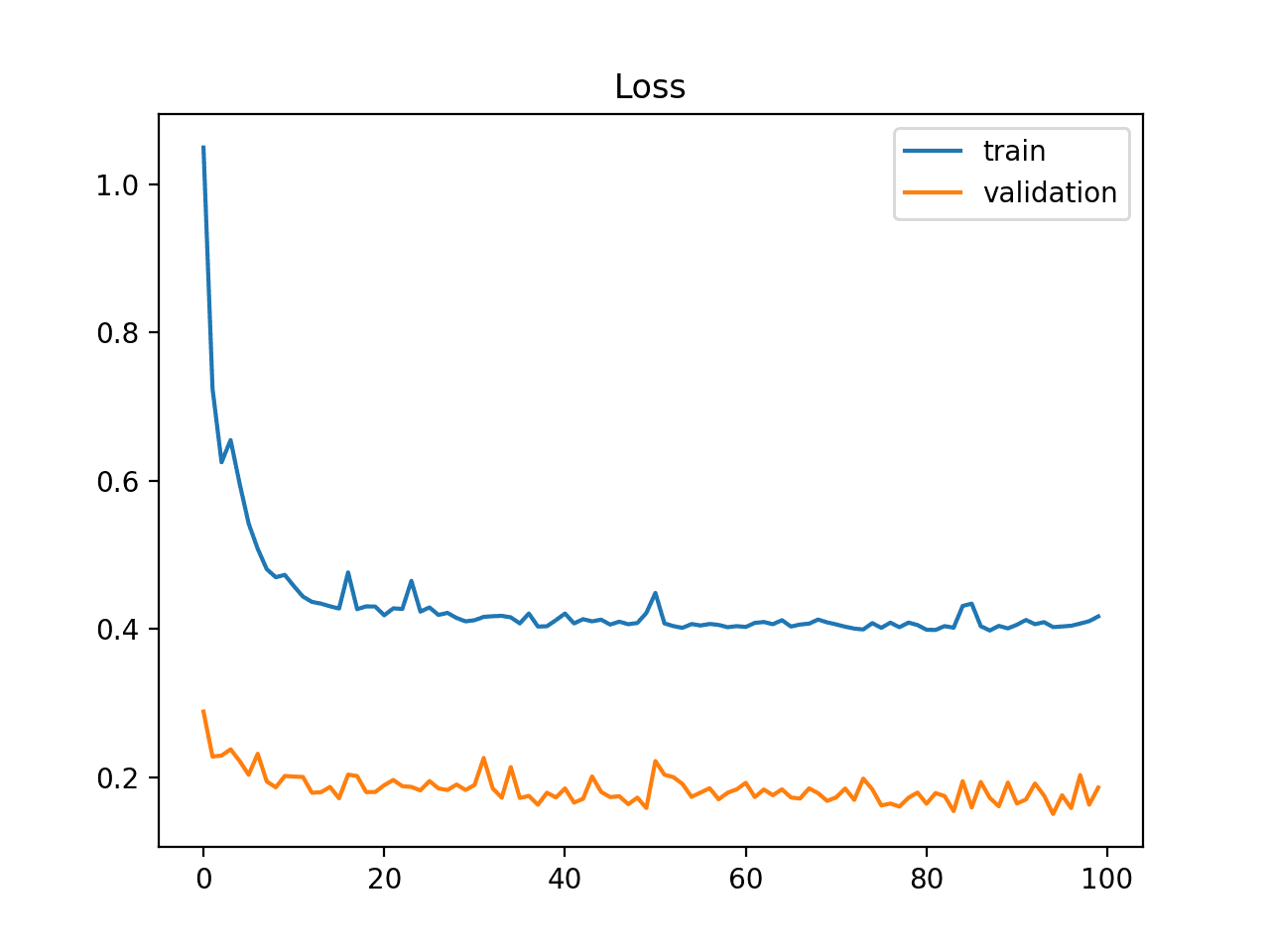### Unrepresentative Validation Dataset An unrepresentative validation dataset means that the validation dataset does not provide sufficient information to evaluate the ability of the model to generalize. This may occur if the validation dataset has too few examples as compared to the training dataset. This case can be identified by a learning curve for training loss that looks like a good fit (or other fits) and a learning curve for validation loss that shows noisy movements around the training loss.  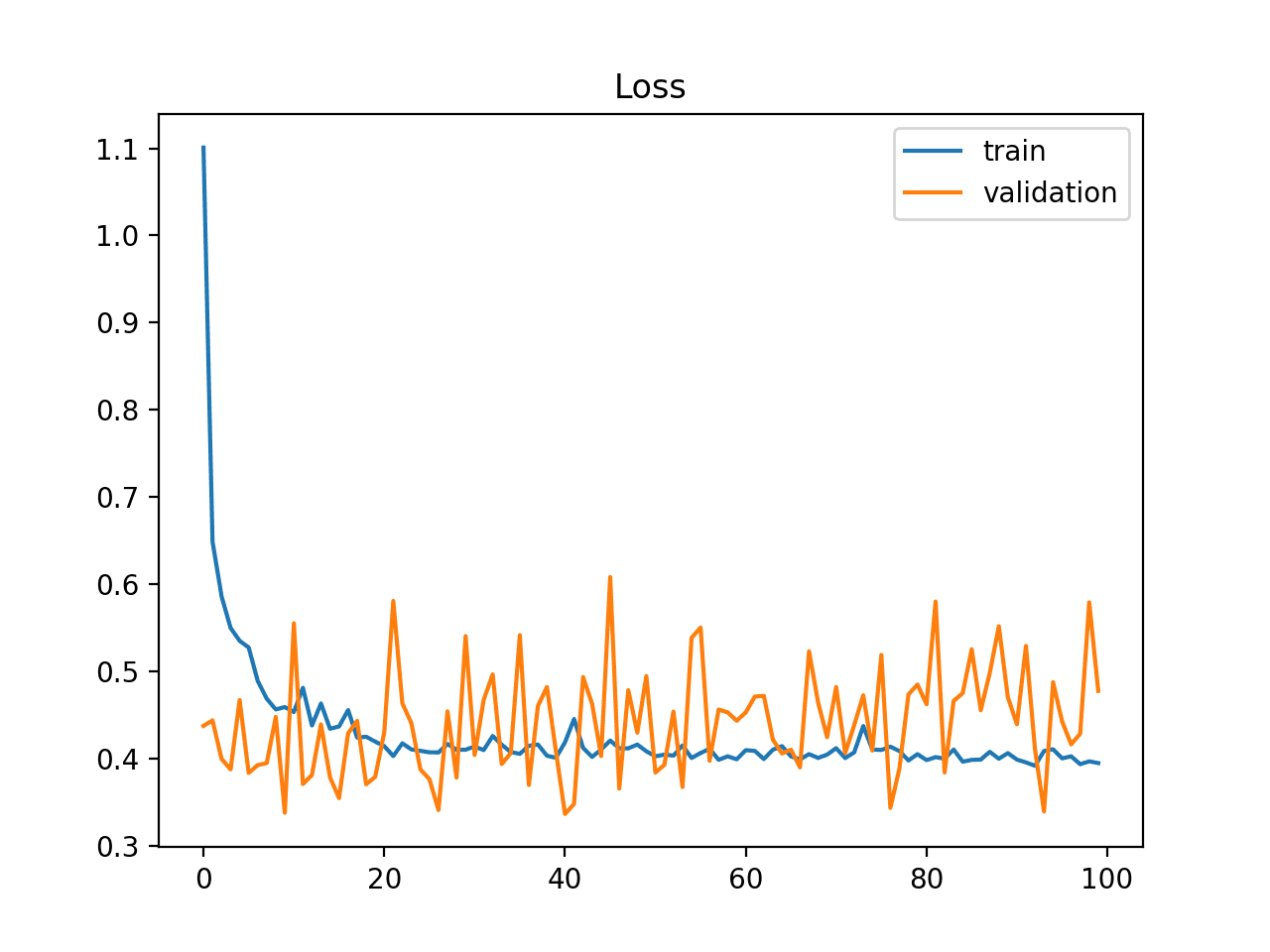This may also be identified by a validation loss that is lower than the training loss which indicates that the validation dataset may be easier for the model to predict than the training dataset.  ## References [1]: [Overfitting and Underfitting Principles](https://towardsdatascience.com/overfitting-and-underfitting-principles-ea8964d9c45c) [2]: [How to Diagnose Overfitting and Underfitting of LSTM Models](https://machinelearningmastery.com/diagnose-overfitting-underfitting-lstm-models/) [3]: [Why is my validation loss lower than my training loss?](https://www.pyimagesearch.com/2019/10/14/why-is-my-validation-loss-lower-than-my-training-loss/) [4]: [How to Mitigate Overfitting with K-Fold Cross-Validation using sklearn](https://towardsdatascience.com/how-to-mitigate-overfitting-with-k-fold-cross-validation-518947ed7428) [5]: [How to use Learning Curves to Diagnose Machine Learning Model Performance](https://machinelearningmastery.com/learning-curves-for-diagnosing-machine-learning-model-performance/) [6]: [Solutions against overfitting for tabular data and classical machine learning](https://towardsdatascience.com/solutions-against-overfitting-for-machine-learning-on-tabular-data-857c080651fd?source=rss----7f60cf5620c9---4)