# Fourier Transform ## Python Signal Processing with scipy.fft - The scipy.fft Module - Install SciPy and Matplotlib - scipy.fft vs scipy.fftpack - scipy.fft vs numpy.fft - The Fourier Transform - When to use the Fourier Transform - Time Domain vs Frequency Domain - Types of Fourier Transforms - Example: Remove Unwanted Noise From Audio - Creating a Signal - Mixing Audio Signals - Using the Fast Fourier Transform (FFT) - Making It Faster With rfft() - Filtering the Signal - Applying the Inverse FFT - Avoiding Filtering Pitfalls - The Discrete Cosine and Sine Transforms ### The Fourier Transform **Fourier analysis** studies how a mathematical function can be decomposed into a series of simpler trigonometric functions. The **Fourier transform** is a tool for decomposing a function into its component frequencies. A **signal** is information that changes over time such as audio, video, and voltage traces. A **frequency** is the speed at which something repeats such as clocks tick at a frequency of one hertz (Hz) or one repetition per second. **Power** refers to the strength of each frequency. Suppose you used the Fourier transform on a recording of someone playing three notes on the piano at the same time. The resulting **frequency spectrum** would show three peaks, one for each of the notes. If the person played one note more softly than the others, then the power of that note’s frequency would be lower than the other two. ### When Do We Need the Fourier Transform In general, we need the Fourier transform if we need to view the frequencies in a signal. If working with a signal in the time domain is difficult, using the Fourier transform to move it into the frequency domain can be helpful. You may have noticed that `fft()` returns a maximum frequency of just over 20 thousand Hertz (22050Hz) which is exactly half of our sampling rate which is called the **Nyquist frequency**. > A fundamental concept in signal processing is the sampling rate must be at least twice the highest frequency in the signal. ### Time Domain vs Frequency Domain We will see the terms time domain and frequency domain. The two terms refer to two different ways of looking at a signal, either as its component frequencies or as information that varies over time. In the **time domain**, a signal is a wave that varies in amplitude (y-axis) over time (x-axis). It is more likely that you are used to seeing graphs in the time domain.  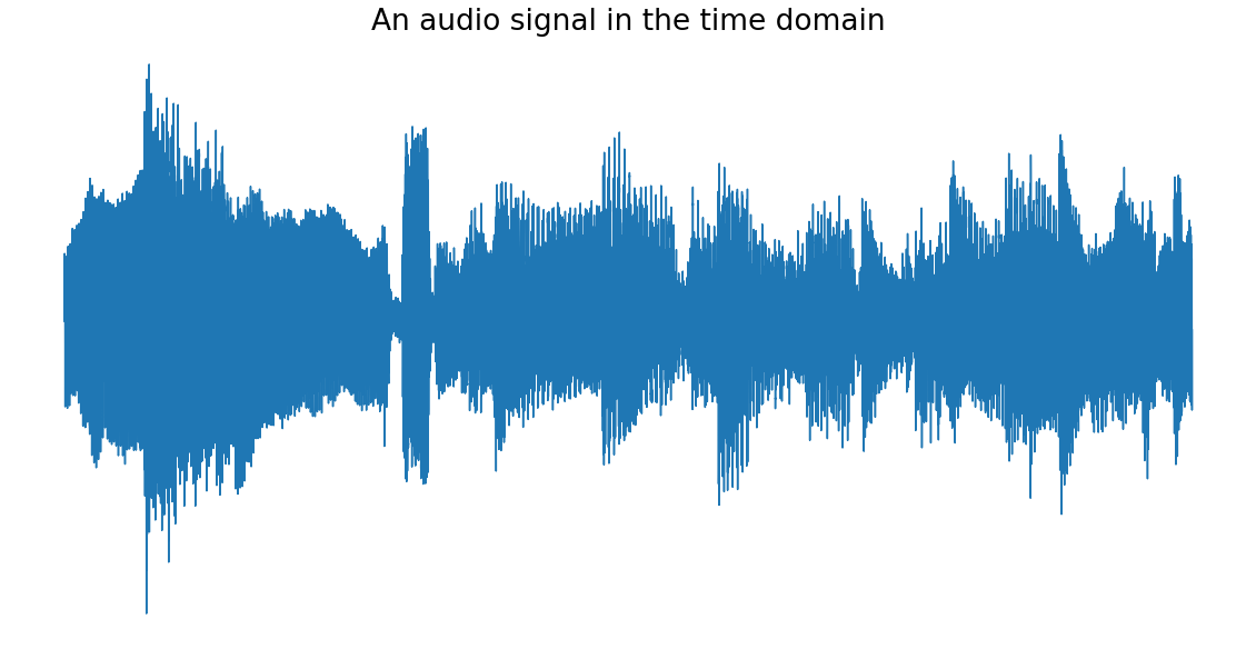In the **frequency domain**, a signal is represented as a series of frequencies (x-axis) that each have an associated power (y-axis). The following image is the above audio signal after being moved to the frequency domain using the Fourier transform:  ### Types of Fourier Transforms The Fourier transform can be subdivided into different types of transform. The most basic subdivision is based on the kind of data the transform operates on: continuous or discrete. This tutorial will deal with only the **discrete Fourier transform (DFT)**. You may see the terms DFT and FFT used interchangeably. However, they are not the same thing. The **fast Fourier transform (FFT)** is an algorithm for computing the discrete Fourier transform (DFT) whereas the DFT is the transform itself. ### Example: Remove Unwanted Noise From Audio To help usbunderstand the Fourier transform, we are going to filter some audio. First, we create an audio signal with a high pitched buzz in it and then we remove the buzz (noise) using the Fourier transform. ### The Discrete Cosine and Sine Transforms A tutorial on the `scipy.fft` module would not be complete without looking at the discrete cosine transform (DCT) and the discrete sine transform (DST). These two transforms are closely related to the Fourier transform but operate entirely on real numbers which means they take a real-valued function as input and produce another real-valued function as output. The DCT and DST are a kina like two halves that together make up the Fourier transform An **even function** is symmetrical about the y-axis whereas an **odd function** is symmetrical about the origin.  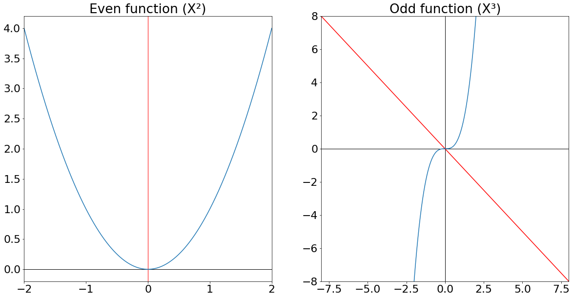Here, the odd function is symmetrical about y = -x which is described as being symmetrical about the origin. When we calculate the Fourier transform, we pretend the function we are calculating it on is infinite. The full Fourier transform (DFT) assumes the input function repeats itself infinitely. However, the DCT and DST assume the function is extended through symmetry. The DCT assumes the function is extended with even symmetry and the DST assumes it is extended with odd symmetry. In the above image, the DFT repeats the function as is whereas the DCT mirrors the function vertically to extend it and the DST mirrors it horizontally. Note that the symmetry implied by the DST leads to big jumps in the function which are called _discontinuities_ and produce more high-frequency components in the resulting frequency spectrum. Therefore, you should use the DCT instead of the DST unless you know your data has odd symmetry. - The DCT is most commonly used. - There are many more examples but the JPEG, MP3, and WebM standards all use the DCT. ---------- ## Understanding Fourier Transform Fourier Transform is a mathematical concept that can convert a continuous signal from time-domain to frequency-domain [2]. ### 1. Reading Audio Files `LibROSA` is a python library that has almost every utility you will need when working with audio data. This rich library comes up with a large number of different functionalities: - Loading and displaying characteristics of an audio file - Spectral representations - Feature extraction and Manipulation - Time-Frequency conversions - Temporal Segmentation - Sequential Modeling Here, we are just going to use a few common features. - Loading Audio - Visualizing Audio The visualization is called the **time-domain** representation of a given signal which shows the loudness (amplitude) of sound wave changing with time. Here, amplitude = 0 represents silence. The amplitudes are not very informative since they only give the loudness of the audio recording. To better understand the audio signal, it is necessary to transform the signal into the frequency-domain. The **frequency-domain** representation of a signal shows the different frequencies that are present in the signal. The Fourier Transform is a mathematical concept that converts a continuous signal from the time-domain to frequency-domain. ### 2. Fourier Transform (FT) An audio signal is a complex signal composed of multiple single-frequency sound waves that travel together as a disturbance(pressure-change) in the medium. When sound is recorded, we only capture the **resultant amplitudes** of those multiple waves. Fourier Transform is a mathematical concept that can **decompose a signal into its constituent frequencies**. Fourier transform does not just give the frequencies present in the signal, it also gives the magnitude of each frequency present in the signal. The **Inverse Fourier Transform** is the opposite of the Fourier Transform which takes the frequency-domain representation of a given signal as input and mathematically synthesizes the original signal.  ### 3. Fast Fourier Transform (FFT) **Fast Fourier Transformation(FFT)** is a mathematical algorithm that calculates the **Discrete Fourier Transform(DFT)** of a given sequence. The only difference between FT(Fourier Transform) and FFT is that FT considers a continuous signal while FFT takes a discrete signal as input. DFT converts a sequence (discrete signal) into its frequency constituents just like FT does for a continuous signal. Here, we have a sequence of amplitudes that were sampled from a continuous audio signal, so the DFT or FFT algorithm can convert this time-domain discrete signal into a frequency-domain. - Simple Sine Wave to Understand FFT - FFT on our Audio signal ### 4. Spectrogram In the previous exercise, we broke our signal into its frequency values which will serve as features for our recognition system. When we applied FFT to our signal, it returned only the frequency values and we lost the the time information. We need to find a way to calculate features for our system such that it has frequency values along with the time at which they were observed which is a **spectrogram**. In a spectrogram plot, one axis represents the time, the second axis represents frequencies, and the colors represent magnitude (amplitude) of the observed frequency at a particular time. Similar to earlier FFT plot, smaller frequencies ranging from (0 – 1kHz) are strong (bright). #### Creating and Plotting the spectrogram The idea is to break the audio signal into smaller frames (windows) and calculate DFT (or FFT) for each window. This way we will be getting frequencies for each window and the window number will represent time. It is a good practice to keep the windows overlapping or we might lose a few frequencies. The window size depends on the problem you are solving. ### 5. Speech Recognition using Spectrogram Features We know how to generate a spectrogram now which is a 2D matrix representing the frequency magnitudes along with time for a given signal. We can think of this spectrogram as an image which reduces it to an **image classification problem**. The image represents the spoken phrase from left to right in a timely manner. Similarly, consider this as an image where the phrase is written from left to right and all we need to do is identify the hidden English characters. Given a parallel corpus of English text, we can train a deep learning model and build a speech recognition system of our own. ## References [1]: [Fourier Transforms with scipy.fft: Python Signal Processing](https://realpython.com/python-scipy-fft/) [2]: [Understanding Audio data, Fourier Transform, FFT, and Spectrogram features for a Speech Recognition System](https://towardsdatascience.com/understanding-audio-data-fourier-transform-fft-spectrogram-and-speech-recognition-a4072d228520) [3]: [Sound Wave Basics](https://dropsofai.com/sound-wave-basics-every-data-scientist-must-know-before-starting-analysis-on-audio-data/)