# Time Series Decomposition ## How to Decompose Time Series Data Time series analysis provides a useful abstraction for selecting forecasting methods which is the _decomposition_ of a time series into systematic and unsystematic components. - **Systematic:** Components of the time series that have consistency or recurrence which can be described and modeled. - **Non-Systematic:** Components of the time series that cannot be directly modeled. A given time series is believed to consist of three systematic components: level, trend, and seasonality plus one non-systematic component called _noise_. - Level: The average value in the series. - Trend: The increasing or decreasing value in the series. - Seasonality: The repeating short-term cycle in the series. - Noise: The random variation in the series. ---------- - Cyclic: A cyclic pattern is a repetitive pattern of the data that does not occur in a fixed period of time which usually repeats more than a year or longer. - Signal: Signal is the real pattern -- the repeatable process/pattern in the data. Thus, Time series analysis is concerned with using methods such as decomposition of a time series into its systematic components in order to understand the underlying causes or the _Why_ behind the time series dataset which is usually not helpful for prediction. ### Combining Time Series Components A time series is assumed to be an aggregate or combination of four components: level, trend, seasonality, and noise. All series have a level and noise, but trend and seasonality components are optional. It is also helpful to think of the components as combining either additive or multiplicative. #### Classical Decomposition The **classical decomposition** (CD) method originated in the 1920s. CD is a relatively simple procedure that is the starting point for most other methods of time series decomposition. There are two forms of classical decomposition: an additive decomposition and a multiplicative decomposition. The classical method of time series decomposition forms the basis of many time series decomposition methods, so it is important to understand how it works. The first step in a classical decomposition is to use a **moving average** method to estimate the trend-cycle. #### Additive Model An additive model suggests that the components are added: ``` y(t) = Level + Trend + Seasonality + Noise ``` An additive model is linear where changes over time are consistently made by the same amount. A linear trend is a straight line. A linear seasonality has the same frequency (width of cycles) and amplitude (height of cycles). #### Multiplicative Model A multiplicative model suggests that the components are multiplied: ``` y(t) = Level * Trend * Seasonality * Noise ``` A multiplicative model is nonlinear () quadratic or exponential) in which changes increase or decrease over time. A nonlinear trend is a curved line. A nonlinear seasonality has an increasing or decreasing frequency and/or amplitude over time. ### Decomposition as a Tool Decomposition is primarily used for time series analysis which can be used to inform forecasting models on the given problem. Decomposition provides a structured way of thinking about a time series forecasting problem, both generally in terms of modeling complexity and specifically in terms of how to best capture each of these components in a given model. Each of these components are something we may need to think about and address during data preparation, model selection, and model tuning. We may address decomposition explicitly in terms of modeling the trend and subtracting it from your data or implicitly by providing enough history for an algorithm to model a trend if it exists. We may or may not be able to cleanly or perfectly break down the time series as an additive or multiplicative model. - Real-world problems are messy and noisy. - There may be additive and multiplicative components. - There may be an increasing trend followed by a decreasing trend. - There may be non-repeating cycles mixed in with the repeating seasonality components. However, these abstract models provide a simple framework that we can use to analyze the data and explore ways to think about and forecast the problem. ### Automatic Time Series Decomposition There are methods to automatically decompose a time series. The `statsmodels` library provides an implementation of the naive or classical decomposition method in a function called `seasonal_decompose()`. The statsmodels linrary requires that we specify whether the model is additive or multiplicative. Both techniques will produce a result and we must be careful to be critical when interpreting the result. A review of a plot of the time series and some summary statistics can often be a good start to get an idea of whether the time series problem appears additive or multiplicative. The `seasonal_decompose()` function returns a result object that contains arrays to access four pieces of data from the decomposition. The snippet below shows how to decompose a series into trend, seasonal, and residual components assuming an additive model: ```py from statsmodels.tsa.seasonal import seasonal_decompose series = ... result = seasonal_decompose(series, model='additive') print(result.trend) print(result.seasonal) print(result.resid) print(result.observed) ``` The result object provides access to the trend and seasonal series as arrays. It also provides access to the _residuals_ which are the time series after the trend and seasonal components are removed. Finally, the original or observed data is also stored. These four time series can be plotted directly from the result object by calling the `plot()` function: ```python from statsmodels.tsa.seasonal import seasonal_decompose from matplotlib import pyplot series = ... result = seasonal_decompose(series, model='additive') result.plot() pyplot.show() ``` Although classical methods are common, they are not recommended for the following reasons: - The technique is not robust to outlier values. - It tends to over-smooth sudden rises and dips in the time series data. - It assumes that the seasonal component repeats from year to year. - The method produces no trend-cycle estimates for the first and last few observations. - There are better methods that can be used for decomposition such as X11 decomposition, SEAT decomposition, or STL decomposition. STL has many advantages over classical, X11, and SEAT decomposition techniques. #### Additive Decomposition ```py from random import randrange from pandas import Series from matplotlib import pyplot from statsmodels.tsa.seasonal import seasonal_decompose series = [i+randrange(10) for i in range(1,100)] result = seasonal_decompose(series, model='additive', period=1) result.plot() pyplot.show() ``` Running the example creates the series, performs the decomposition, and plots the 4 resulting series. We can see that the entire series was taken as the trend component and that there was no seasonality. We can also see that the residual plot shows zero which is a good example where the naive or classical decomposition was not able to separate the noise that we added from the linear trend. There are more advanced decompositions available such Seasonal and Trend decomposition using Loess or STL decomposition. #### Multiplicative Decomposition We can contrive a quadratic time series as a square of the time step from 1 to 99, and then decompose it assuming a multiplicative model. Running the example, we can see that, as in the additive case, the trend is easily extracted and wholly characterizes the time series. ```py from pandas import Series from matplotlib import pyplot from statsmodels.tsa.seasonal import seasonal_decompose series = [i**2.0 for i in range(1,100)] result = seasonal_decompose(series, model='multiplicative', period=1) result.plot() pyplot.show() ``` Exponential changes can be made linear by data transforms. Here, a quadratic trend can be made linear by applying the square root. An exponential growth in seasonality can be made linear by taking the natural logarithm. Again, it is important to treat decomposition as a potentially useful analysis tool, but consider exploring the many different ways it could be applied to your problem such as on data after it has been transformed or on residual model errors. ### Airline Passengers Dataset The airline passengers dataset describes the total number of airline passengers over a period of time. The units are a count of the number of airline passengers in thousands. There are 144 monthly observations from 1949 to 1960. First, we graph the raw observations. ```py from pandas import read_csv from matplotlib import pyplot series = read_csv('airline-passengers.csv', header=0, index_col=0) series.plot() pyplot.show() ``` Reviewing the line plot, it suggests that there may be a linear trend but it is hard to be sure just by eye-balling. There is also seasonality, but the amplitude (height) of the cycles appears to be increasing, suggesting that it is multiplicative. Thus, we will assume a multiplicative model. The example below decomposes the airline passenger dataset as a multiplicative model. ```py from pandas import read_csv from matplotlib import pyplot from statsmodels.tsa.seasonal import seasonal_decompose series = read_csv('airline-passengers.csv', header=0, index_col=0) result = seasonal_decompose(series, model='multiplicative') result.plot() pyplot.show() ``` Running the example plots the observed, trend, seasonal, and residual time series.  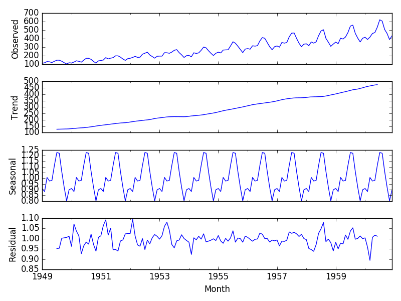We can see that the trend and seasonality information extracted from the series does seem reasonable. The residuals also show periods of high variability in the early and later years of the series. ---------- ## Time Series 101 Guide ### STL Decomposition STL stands for seasonal and trend decomposition using Loess. STL is robust to outliers and can handle any kind of seasonality which also makes it a versatile method for decomposition. There are a few things we can control when using STL: - Trend cycle smoothness - Rate of change in seasonal component - The robustness towards the user outlier or exceptional values which controls the effects of outliers on the seasonal and trend components. SLT has some disadvantages: - STL cannot handle calendar variations automatically. - STL only provides a decomposition for additive models. We can obtain the multiplicative decomposition by taking the logarithm of the data and then transforming the components. ```py import pandas as pd import seaborn as sns import matplotlib.pyplot as plt from statsmodels.tsa.seasonal import STL elec_equip = read_csv(r"C:/Users/datas/python/data/elecequip.csv") stl = STL(elec_equip, period=12, robust=True) res_robust = stl.fit() fig = res_robust.plot() ``` ### Basic Time Series Forecasting Methods Although there are many statistical techniques for forecasting time series data, here we only consider the most straight-forward and simple methods that can be used for effective time series forecasting. These methods also serve as the foundation for some of the other methods: - Simple Moving Average (SMA) - Weighted Moving Average (WMA) - Exponential Moving Average (EMA) ---------- ## How to isolate trend, seasonality, and noise from a time series The commonly occurring seasonal periods are a day, week, month, quarter (or season), and year. ### The Seasonal component The seasonal component explains the periodic ups and downs one sees in many data sets such as the one shown below. Seasonality can also observed on much longer time scales such as in the solar cycle which follows a roughly 11 year period. ### The Trend component The Trend component refers to the pattern in the data that spans across seasonal periods. The time series of retail eCommerce sales shown below demonstrates a possibly quadratic trend (y = x²) that spans across the 12 month long seasonal period: ### The Cyclical component The cyclical component represents phenomena that happen across seasonal periods. Cyclical patterns do not have a fixed period like seasonal patterns. An example of a cyclical pattern is the cycles of boom and bust that stock markets experience in response to world events. The cyclical component is hard to isolate, so it is often left alone by combining it with the trend component. ### The Noise component The noise or random component is what remains after we separate the seasonality and trend from the time series. Noise is the effect of factors that you do not know or we cannot measure. Noise is the effect of the known unknowns or the unknown unknowns. ### Additive and Multiplicative effects The trend, seasonal and noise components can combine in an additive or a multiplicative way. ### Decomposing a time series into trend, seasonal, and noise components There are many decomposition methods available ranging from simple moving average based methods to powerful ones such as STL. We can create the decomposition of a time series into its trend, seasonal, and noise components using a simple procedure based on moving averages: STEP 1: Identify the length of the seasonal period STEP 2: Isolate the trend STEP 3: Isolate the seasonality + noise STEP 4: Isolate the seasonality STEP 5: Isolate the noise ### Time series decomposition using statsmodels Now that we know how decomposition works, we can use the `seasonal_decompose()` in statsmodels to perform all of the work in one line of code: ```py from statsmodels.tsa.seasonal import seasonal_decompose components = seasonal_decompose(df['Retail_Sales'], model='multiplicative') # components = seasonal_decompose(np.array(elecequip), model='multiplicative', freq=4) components.plot() ``` ---------- ## Avoid Common Mistakes Here are some common mistakes to avoid with time series forecasting [8]: - How to find peaks and troughs in a time series signal? - What is (and how to use) autocorrelation plot? - How to check if a time series has any statistically significant signal? ## References [1]: [How to Decompose Time Series Data into Trend and Seasonality](https://machinelearningmastery.com/decompose-time-series-data-trend-seasonality/) [2]: [Time Series Forecast and Decomposition 101 Guide Python](https://datasciencebeginners.com/2020/11/25/time-series-forecast-and-decomposition-101-guide-python/) [3]: [How To Isolate Trend, Seasonality, and Noise From A Time Series](https://timeseriesreasoning.com/contents/time-series-decomposition/) [4]: [Avoid These Mistakes with Time Series Forecasting](https://www.kdnuggets.com/2021/12/avoid-mistakes-time-series-forecasting.html)